This semester at uni I’ve been doing a capstone project (an iLab). Due to the volume of data, I’ve slapped it into a local MySQL instance (as I already had MySQL installed). To get the dataset down to a manageable size before loading it into R, I’ve been toying around with tidyverse’s dbplyr. It uses the same standard approach as the rest of the tidyverse family, something I’m already comfortable with.

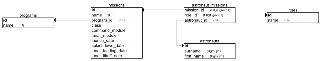
This post does assume some familiarity with SQL. Rather than risk violating my client’s non-disclosure agreement, I’ve created a small database of the early days of NASA, with the following structure:

If you want to follow along, the code to create and populate the MySQL database is here, and the R code is here. In both cases, change the password from xxxxxxxx to something more secure.

You’ll need to install the dbplyr dbplyr package too.

Connecting to the database

# Connect to the database (MYSQL* constants have been previously defined)
dbcon <- src_mysql(
dbname = MYSQL_DB,
host = MYSQL_HOST,
port = MYSQL_PORT,
user = MYSQL_USER,
password = MYSQL_PASS)

# Create references to our database tables (TABLE_NAME_* constants are strings already defined)
programs <- tbl(dbcon, TABLE_NAME_PROGRAMS)
astronauts <- tbl(dbcon, TABLE_NAME_ASTRONAUTS)
missions <- tbl(dbcon, TABLE_NAME_MISSIONS)
roles <- tbl(dbcon, TABLE_NAME_ROLES)
astronaut_missions <- tbl(dbcon, TABLE_NAME_ASTRONAUT_MISSIONS)

Lazy loading

Once defined, our tbls can be used much like any other R dataframe.

There are, however, a few things to be aware of. First, the tbls don’t contain the complete dataset at this point – it’s easier to think of them as promises to fetch the data from the database when needed. Looking more closely at the tbl makes this clearer:

str(astronauts)

## List of 2
## $ src:List of 2
## ..$ con :Formal class 'MySQLConnection' [package "RMySQL"] with 1 slot
## .. .. ..@ Id: int [1:2] 0 0
## ..$ disco:
## ..- attr(*, "class")= chr [1:3] "src_dbi" "src_sql" "src"
## $ ops:List of 2
## ..$ x :Classes 'ident', 'character' chr "astronauts"
## ..$ vars: chr [1:3] "id" "surname" "first_name"
## ..- attr(*, "class")= chr [1:3] "op_base_remote" "op_base" "op"
## - attr(*, "class")= chr [1:4] "tbl_dbi" "tbl_sql" "tbl_lazy" "tbl"

 

We see it’s not a standard R dataframe, but an implementation of tbl called tbl_lazy . It’s the “lazy” part of the name that signifies the data won’t be loaded until required.

Generated SQL

The show_query()  function illustrates exactly what form the SQL will take when it’s run. For example:

show_query(astronauts)
## <SQL>
## SELECT *
## FROM `astronauts`

or

astronauts %>%
count() %>%
show_query()

## <SQL>
## SELECT count(*) AS `n`
## FROM `astronauts`

 

As the second example shows, dbplyr  will convert chained commands into a single piece of SQL where possible, having the database do the work, rather than retrieving data into memory and manipulating it there.

Examining the data

As mentioned, dbplyr  won’t fetch the data from the database until it’s needed. But it will pull in a little so we can examine the data. For example, looking at the astronauts tbl :

astronauts
## # Source: table [?? x 3]
## # Database: mysql 5.7.11-log [nasa@localhost:/nasa]
## id surname first_name
##
## 1 19 Aldrin Buzz
## 2 23 Anders Bill
## 3 14 Armstrong Neil
## 4 25 Bean Alan
## 5 12 Borman Frank
## 6 4 Carpenter Scott
## 7 16 Cernan Eugene
## 8 20 Chaffee Roger
## 9 17 Collins Michael
## 10 10 Conrad Pete
## # ... with more rows

Note that the first line says [?? x 3] , and the last line says # … with more rows , without specifying how many more rows. These are both indications that the full query hasn’t been run. In fact, looking at the database logs, the query that has been run is SELECT * FROM “astronauts“ LIMIT 10 . The use of the limit clause is dbplyr ’s way of getting enough data to display, without needing to pull in all the data.

Note that the glimpse()  function in the dplyr  package isn’t quite as helpful:

glimpse(astronauts)
## Observations: 25
## Variables: 3
## $ id 19, 23, 14, 25, 12, 4, 16, 20, 17, 10, 6, 22, 33, 2...
## $ surname "Aldrin", "Anders", "Armstrong", "Bean", "Borman", ...
## $ first_name "Buzz", "Bill", "Neil", "Alan", "Frank", "Scott", "...

Observations: 25  gives the impression that the size of the dataset is known, where it is not. This time, the database logs show SELECT * FROM “astronauts“ LIMIT 25 , and

astronauts %>%
count() %>%
collect()

## # A tibble: 1 x 1
## n
##
## 1 35

shows there are in fact 35 astronauts in the table.

Forcing data to be loaded

The previous command shows how to force R to load the data into memory: the collect()  function. It converts the promise of data into a concrete data frame. Compare

str(astronauts)
## List of 2
## $ src:List of 2
## ..$ con :Formal class 'MySQLConnection' [package "RMySQL"] with 1 slot
## .. .. ..@ Id: int [1:2] 0 0
## ..$ disco:
## ..- attr(*, "class")= chr [1:3] "src_dbi" "src_sql" "src"
## $ ops:List of 2
## ..$ x :Classes 'ident', 'character' chr "astronauts"
## ..$ vars: chr [1:3] "id" "surname" "first_name"
## ..- attr(*, "class")= chr [1:3] "op_base_remote" "op_base" "op"
## - attr(*, "class")= chr [1:4] "tbl_dbi" "tbl_sql" "tbl_lazy" "tbl"

with

str(astronauts %>% collect())
## Classes 'tbl_df', 'tbl' and 'data.frame': 35 obs. of 3 variables:
## $ id : int 19 23 14 25 12 4 16 20 17 10 ...
## $ surname : chr "Aldrin" "Anders" "Armstrong" "Bean" ...
## $ first_name: chr "Buzz" "Bill" "Neil" "Alan" ...

Complex queries

As mentioned above, dbplyr  will try to do as much processing as possible in the database. For example, in order to determine the astronauts who flew multiple missions in Gemini or Apollo, you’d do something like this with dplyr:

multiple_missions <- astronaut_missions %>%
    inner_join(missions, by=c("mission_id" = "id"), suffix = c("_am", "_m")) %>%
    inner_join(programs, by=c("program_id" = "id"), suffix = c("_m", "_p")) %>%
    filter(name_p %in% c("Gemini", "Apollo")) %>%
    group_by(name_p, astronaut_id) %>%
    summarise(flights = n()) %>%
    ungroup() %>%
    filter(flights >= 2) %>%
    inner_join(astronauts, by=c("astronaut_id" = "id"), suffix = c("_am", "_a")) %>%
    arrange(desc(flights), name_p, surname, first_name) %>%
    select(program_name = name_p, surname, first_name, flights)

 

multiple_missions

## # Source: lazy query [?? x 4]
## # Database: mysql 5.7.11-log [nasa@localhost:/nasa]
## # Ordered by: desc(flights), name_p, surname, first_name
## program_name surname first_name flights
##
## 1 Apollo Cernan Eugene 2
## 2 Apollo Lovell Jim 2
## 3 Apollo Scott David 2
## 4 Apollo Young John 2
## 5 Gemini Conrad Pete 2
## 6 Gemini Lovell Jim 2
## 7 Gemini Stafford Tom 2
## 8 Gemini Young John 2

 

Looking at how dbplyr  handles this, we find it’s all pushed into the database, and run as a single query:

multiple_missions %>%
    show_query()

 

## <SQL>
## SELECT `name_p` AS `program_name`, `surname` AS `surname`, `first_name` AS `first_name`, `flights` AS `flights`
## FROM (SELECT *
## FROM (SELECT `TBL_LEFT`.`name_p` AS `name_p`, `TBL_LEFT`.`astronaut_id` AS `astronaut_id`, `TBL_LEFT`.`flights` AS `flights`, `TBL_RIGHT`.`surname` AS `surname`, `TBL_RIGHT`.`first_name` AS `first_name`
## FROM (SELECT *
## FROM (SELECT `name_p`, `astronaut_id`, count(*) AS `flights`
## FROM (SELECT *
## FROM (SELECT `TBL_LEFT`.`mission_id` AS `mission_id`, `TBL_LEFT`.`role_id` AS `role_id`, `TBL_LEFT`.`astronaut_id` AS `astronaut_id`, `TBL_LEFT`.`name` AS `name_m`, `TBL_LEFT`.`program_id` AS `program_id`, `TBL_LEFT`.`class` AS `class`, `TBL_LEFT`.`command_module` AS `command_module`, `TBL_LEFT`.`lunar_module` AS `lunar_module`, `TBL_LEFT`.`launch_date` AS `launch_date`, `TBL_LEFT`.`splashdown_date` AS `splashdown_date`, `TBL_LEFT`.`lunar_landing_date` AS `lunar_landing_date`, `TBL_LEFT`.`lunar_liftoff_date` AS `lunar_liftoff_date`, `TBL_RIGHT`.`name` AS `name_p`
## FROM (SELECT `TBL_LEFT`.`mission_id` AS `mission_id`, `TBL_LEFT`.`role_id` AS `role_id`, `TBL_LEFT`.`astronaut_id` AS `astronaut_id`, `TBL_RIGHT`.`name` AS `name`, `TBL_RIGHT`.`program_id` AS `program_id`, `TBL_RIGHT`.`class` AS `class`, `TBL_RIGHT`.`command_module` AS `command_module`, `TBL_RIGHT`.`lunar_module` AS `lunar_module`, `TBL_RIGHT`.`launch_date` AS `launch_date`, `TBL_RIGHT`.`splashdown_date` AS `splashdown_date`, `TBL_RIGHT`.`lunar_landing_date` AS `lunar_landing_date`, `TBL_RIGHT`.`lunar_liftoff_date` AS `lunar_liftoff_date`
## FROM `astronaut_missions` AS `TBL_LEFT`
## INNER JOIN `missions` AS `TBL_RIGHT`
## ON (`TBL_LEFT`.`mission_id` = `TBL_RIGHT`.`id`)
## ) `TBL_LEFT`
## INNER JOIN `programs` AS `TBL_RIGHT`
## ON (`TBL_LEFT`.`program_id` = `TBL_RIGHT`.`id`)
## ) `mcqvbvfalf`
## WHERE (`name_p` IN ('Gemini', 'Apollo'))) `gnbzqrugnr`
## GROUP BY `name_p`, `astronaut_id`) `jsfgxpaqfn`
## WHERE (`flights` >= 2.0)) `TBL_LEFT`
## INNER JOIN `astronauts` AS `TBL_RIGHT`
## ON (`TBL_LEFT`.`astronaut_id` = `TBL_RIGHT`.`id`)
## ) `bnlhfwyrus`
## ORDER BY `flights` DESC, `name_p`, `surname`, `first_name`) `zhxhmqlgye`

 

A big, ugly, query to be sure. And while I could write it more succinctly by hand, I’ve found the query plans are identical, and I need not use SQL if I already know dplyr .

Gotchas

dplyr  users will find it’s not a completely painless transition to dbplyr  however. Take, for example, finding all the astronauts whose surnames start with “C”. In dplyr , you might use something like:

astronauts %>%
    filter(grepl("^C", surname))

Unfortunately, this will return an error reporting that FUNCTION nasa.GREPL does not exist .

One alternative is to collect()  the data before applying the filter:

astronauts %>%
    collect() %>%
    filter(grepl("^C", surname))

That may not be efficient if we’re doing a lot of processing after the filter()  command, and it flies in the face of our goal to do as much processing as possible in the database.

In this case, we’d like to use the SQL LIKE  operator. We could guess that something like filter(surname %like% ‘C%’)  might do the trick. Rather than running the full (possibly expensive) query, we can use dbplyr ’s translate_sql()  function, which will show how an R command will be converted to SQL. For example:

dbplyr::translate_sql(x == 1 && (y 3))
## <SQL> "x" = 1.0 AND ("y" 3.0)

If translate_sql()  doesn’t know what to do with a piece of code, it’ll pass the code to the database more or less as is. This was the cause of the FUNCTION nasa.GREPL does not exist  error we got above:

dbplyr::translate_sql(grepl("^C", surname))
## <SQL> GREPL('^C', "surname")

But it does mean that even if translate_sql()  doesn’t know about the SQL LIKE  operator, our guess of filter(surname %like% ‘C%’)  will be passed through to the database as we need:

dbplyr::translate_sql(surname %like% 'C%')
## <SQL> "surname" LIKE 'C%'

 

astronauts %>%
filter(surname %like% 'C%')

## # Source: lazy query [?? x 3]
## # Database: mysql 5.7.11-log [nasa@localhost:/nasa]
## id surname first_name
##
## 1 4 Carpenter Scott
## 2 16 Cernan Eugene
## 3 20 Chaffee Roger
## 4 17 Collins Michael
## 5 10 Conrad Pete
## 6 6 Cooper Gordo
## 7 22 Cunningham Walt

 

Query plans

As well as show_query() , dbplyr  provides the explain()  function, which gives detail about how the database optimiser will run the query. This is useful to check that (for example) the database will make efficient use of indices.

astronauts %>%
    filter(surname %like% 'C%') %>%
    explain()

 

## <SQL>
## SELECT *
## FROM `astronauts`
## WHERE (`surname` LIKE 'C%')

##

## <PLAN>
## id select_type table partitions type possible_keys key
## 1 1 SIMPLE astronauts range astronaut_name astronaut_name
## key_len ref rows filtered Extra
## 1 62 7 100 Using where; Using index